Time and Dates (`astropy.time`)¶

Introduction¶

The astropy.time package provides functionality for manipulating times and dates. Specific emphasis is placed on supporting time scales (e.g. UTC, TAI, UT1, TDB) and time representations (e.g. JD, MJD, ISO 8601) that are used in astronomy and required to calculate, e.g., sidereal times and barycentric corrections. It uses Cython to wrap the C language ERFA time and calendar routines, using a fast and memory efficient vectorization scheme.

All time manipulations and arithmetic operations are done internally using two 64-bit floats to represent time. Floating point algorithms from [1] are used so that the Time object maintains sub-nanosecond precision over times spanning the age of the universe.

[1]	Shewchuk, 1997, Discrete & Computational Geometry 18(3):305-363

Getting Started¶

The basic way to use astropy.time is to create a Time object by supplying one or more input time values as well as the time format and time scale of those values. The input time(s) can either be a single scalar like "2010-01-01 00:00:00" or a list or a numpy array of values as shown below. In general any output values have the same shape (scalar or array) as the input.

>>> from astropy.time import Time
>>> times = ['1999-01-01T00:00:00.123456789', '2010-01-01T00:00:00']
>>> t = Time(times, format='isot', scale='utc')
>>> t
<Time object: scale='utc' format='isot' value=['1999-01-01T00:00:00.123' '2010-01-01T00:00:00.000']>
>>> t[1]
<Time object: scale='utc' format='isot' value=2010-01-01T00:00:00.000>

The format argument specifies how to interpret the input values, e.g. ISO or JD or Unix time. The scale argument specifies the time scale for the values, e.g. UTC or TT or UT1. The scale argument is optional and defaults to UTC except for Time from epoch formats. We could have written the above as:

>>> t = Time(times, format='isot')

When the format of the input can be unambiguously determined then the format argument is not required, so we can simplify even further:

>>> t = Time(times)

Now let’s get the representation of these times in the JD and MJD formats by requesting the corresponding Time attributes:

>>> t.jd
array([ 2451179.50000143,  2455197.5       ])
>>> t.mjd
array([ 51179.00000143,  55197.        ])

We can also convert to a different time scale, for instance from UTC to TT. This uses the same attribute mechanism as above but now returns a new Time object:

>>> t2 = t.tt
>>> t2
<Time object: scale='tt' format='isot' value=['1999-01-01T00:01:04.307' '2010-01-01T00:01:06.184']>
>>> t2.jd
array([ 2451179.5007443 ,  2455197.50076602])

Note that both the ISO (ISOT) and JD representations of t2 are different than for t because they are expressed relative to the TT time scale.

Finally, some further examples of what is possible. For details, see the API documentation below.

>>> dt = t[1] - t[0]
>>> dt
<TimeDelta object: scale='tai' format='jd' value=4018.0000217...>

Here, note the conversion of the timescale to TAI. Time differences can only have scales in which one day is always equal to 86400 seconds.

>>> import numpy as np
>>> t[0] + dt * np.linspace(0.,1.,12)
<Time object: scale='utc' format='isot' value=['1999-01-01T00:00:00.123' '2000-01-01T06:32:43.930'
 '2000-12-31T13:05:27.737' '2001-12-31T19:38:11.544'
 '2003-01-01T02:10:55.351' '2004-01-01T08:43:39.158'
 '2004-12-31T15:16:22.965' '2005-12-31T21:49:06.772'
 '2007-01-01T04:21:49.579' '2008-01-01T10:54:33.386'
 '2008-12-31T17:27:17.193' '2010-01-01T00:00:00.000']>

>>> t.sidereal_time('apparent', 'greenwich')
<Longitude [ 6.68050179, 6.70281947] hourangle>

Using `astropy.time`¶

Time object basics¶

In astropy.time a “time” is a single instant of time which is independent of the way the time is represented (the “format”) and the time “scale” which specifies the offset and scaling relation of the unit of time. There is no distinction made between a “date” and a “time” since both concepts (as loosely defined in common usage) are just different representations of a moment in time.

Once a Time object is created it cannot be altered internally. In code lingo it is “immutable.” In particular the common operation of “converting” to a different time scale is always performed by returning a copy of the original Time object which has been converted to the new time scale.

Time Format¶

The time format specifies how an instant of time is represented. The currently available formats are can be found in the Time.FORMATS dict and are listed in the table below. Each of these formats is implemented as a class that derives from the base TimeFormat class. This class structure can be easily adapted and extended by users for specialized time formats not supplied in astropy.time.

Format	Class	Example argument
byear	`TimeBesselianEpoch`	1950.0
byear_str	`TimeBesselianEpochString`	‘B1950.0’
cxcsec	`TimeCxcSec`	63072064.184
datetime	`TimeDatetime`	datetime(2000, 1, 2, 12, 0, 0)
gps	`TimeGPS`	630720013.0
iso	`TimeISO`	‘2000-01-01 00:00:00.000’
isot	`TimeISOT`	‘2000-01-01T00:00:00.000’
jd	`TimeJD`	2451544.5
jyear	`TimeJulianEpoch`	2000.0
jyear_str	`TimeJulianEpochString`	‘J2000.0’
mjd	`TimeMJD`	51544.0
plot_date	`TimePlotDate`	730120.0003703703
unix	`TimeUnix`	946684800.0
yday	`TimeYearDayTime`	2000:001:00:00:00.000

Subformat¶

The time format classes TimeISO, TimeISOT, and TimeYearDayTime support the concept of subformats. This allows for variations on the basic theme of a format in both the input string parsing and the output.

The supported subformats are date_hms, date_hm, and date. The table below illustrates these subformats for iso and yday formats:

Format	Subformat	Input / output
`iso`	date_hms	2001-01-02 03:04:05.678
`iso`	date_hm	2001-01-02 03:04
`iso`	date	2001-01-02
`yday`	date_hms	2001:032:03:04:05.678
`yday`	date_hm	2001:032:03:04
`yday`	date	2001:032

Time from epoch formats¶

The formats cxcsec, gps, and unix are a little special in that they provide a floating point representation of the elapsed time in seconds since a particular reference date. These formats have a intrinsic time scale which is used to compute the elapsed seconds since the reference date.

Format	Scale	Reference date
`cxcsec`	TT	`1998-01-01 00:00:00`
`unix`	UTC	`1970-01-01 00:00:00`
`gps`	TAI	`1980-01-06 00:00:19`

Unlike the other formats which default to UTC, if no scale is provided when initializing a Time object then the above intrinsic scale is used. This is done for computational efficiency.

Time Scale¶

The time scale (or time standard) is “a specification for measuring time: either the rate at which time passes; or points in time; or both” [2]. See also [3] and [4].

>>> Time.SCALES
('tai', 'tcb', 'tcg', 'tdb', 'tt', 'ut1', 'utc')

Scale	Description
tai	International Atomic Time (TAI)
tcb	Barycentric Coordinate Time (TCB)
tcg	Geocentric Coordinate Time (TCG)
tdb	Barycentric Dynamical Time (TDB)
tt	Terrestrial Time (TT)
ut1	Universal Time (UT1)
utc	Coordinated Universal Time (UTC)

[2]	Wikipedia time standard article

[3]	SOFA Time Scale and Calendar Tools (PDF)

[4]	http://www.ucolick.org/~sla/leapsecs/timescales.html

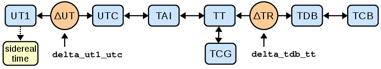
The system of transformation between supported time scales is shown in the figure below. Further details are provided in the Convert time scale section.

Scalar or Array¶

A Time object can hold either a single time value or an array of time values. The distinction is made entirely by the form of the input time(s). If a Time object holds a single value then any format outputs will be a single scalar value, and likewise for arrays. Like other arrays and lists, Time objects holding arrays are subscriptable, returning scalar or array objects as appropriate:

>>> from astropy.time import Time
>>> t = Time(100.0, format='mjd')
>>> t.jd
2400100.5
>>> t = Time([100.0, 200.0, 300.], format='mjd')
>>> t.jd
array([ 2400100.5,  2400200.5,  2400300.5])
>>> t[:2]
<Time object: scale='utc' format='mjd' value=[ 100.  200.]>
>>> t[2]
<Time object: scale='utc' format='mjd' value=300.0>

Inferring input format¶

The Time class initializer will not accept ambiguous inputs, but it will make automatic inferences in cases where the inputs are unambiguous. This can apply when the times are supplied as datetime objects or strings. In the latter case it is not required to specify the format because the available string formats have no overlap. However, if the format is known in advance the string parsing will be faster if the format is provided.

>>> from datetime import datetime
>>> t = Time(datetime(2010, 1, 2, 1, 2, 3))
>>> t.format
'datetime'
>>> t = Time('2010-01-02 01:02:03')
>>> t.format
'iso'

Internal representation¶

The Time object maintains an internal representation of time as a pair of double precision numbers expressing Julian days. The sum of the two numbers is the Julian Date for that time relative to the given time scale. Users requiring no better than microsecond precision over human time scales (~100 years) can safely ignore the internal representation details and skip this section.

This representation is driven by the underlying ERFA C-library implementation. The ERFA routines take care throughout to maintain overall precision of the double pair. The user is free to choose the way in which total JD is provided, though internally one part contains integer days and the other the fraction of the day, as this ensures optimal accuracy for all conversions. The internal JD pair is available via the jd1 and jd2 attributes:

>>> t = Time('2010-01-01 00:00:00', scale='utc')
>>> t.jd1, t.jd2
(2455197.5, 0.0)
>>> t2 = t.tai
>>> t2.jd1, t2.jd2
(2455197.5, 0.00039351851851851...)

Creating a Time object¶

The allowed Time arguments to create a time object are listed below:

val : numpy ndarray, list, str, or number: Data to initialize table.
val2 : numpy ndarray, list, str, or number; optional: Data to initialize table.
format : str, optional: Format of input value(s)
scale : str, optional: Time scale of input value(s)
precision : int between 0 and 9 inclusive: Decimal precision when outputting seconds as floating point
in_subfmt : str: Unix glob to select subformats for parsing string input times
out_subfmt : str: Unix glob to select subformats for outputting string times
location : EarthLocation or tuple, optional: If a tuple, 3 Quantity items with length units for geocentric coordinates, or a longitude, latitude, and optional height for geodetic coordinates. Can be a single location, or one for each input time.

val¶

The val argument specifies the input time or times and can be a single string or number, or it can be a Python list or numpy array of strings or numbers. To initialize a Time object based on a specified time, it must be present. If val is absent (or None), the Time object will be created for the time corresponding to the instant the object is created.

In most situations one also needs to specify the time scale via the scale argument. The Time class will never guess the time scale, so a simple example would be:

>>> t1 = Time(50100.0, scale='tt', format='mjd')
>>> t2 = Time('2010-01-01 00:00:00', scale='utc')

It is possible to create a new Time object from one or more existing time objects. In this case the format and scale will be inferred from the first object unless explicitly specified.

>>> Time([t1, t2])
<Time object: scale='tt' format='mjd' value=[ 50100.  55197.00076602]>

val2¶

The val2 argument is available for specialized situations where extremely high precision is required. Recall that the internal representation of time within astropy.time is two double-precision numbers that when summed give the Julian date. If provided the val2 argument is used in combination with val to set the second the internal time values. The exact interpretation of val2 is determined by the input format class. As of this release all string-valued formats ignore val2 and all numeric inputs effectively add the two values in a way that maintains the highest precision. Example:

>>> t = Time(100.0, 0.000001, format='mjd', scale='tt')
>>> t.jd, t.jd1, t.jd2  
(2400100.50000..., 2400100.5, 1e-06)

format¶

The format argument sets the time time format, and as mentioned it is required unless the format can be unambiguously determined from the input times.

scale¶

The scale argument sets the time scale and is required except for time formats such as plot_date (TimePlotDate) and unix (TimeUnix). These formats represent the duration in SI seconds since a fixed instant in time which is independent of time scale.

precision¶

The precision setting affects string formats when outputting a value that includes seconds. It must be an integer between 0 and 9. There is no effect when inputting time values from strings. The default precision is 3. Note that the limit of 9 digits is driven by the way that ERFA handles fractional seconds. In practice this should should not be an issue.

>>> t = Time('B1950.0', scale='utc', precision=3)
>>> t.byear_str
'B1950.000'
>>> t.precision = 0
>>> t.byear_str
'B1950'

in_subfmt¶

The in_subfmt argument provides a mechanism to select one or more subformat values from the available subformats for string input. Multiple allowed subformats can be selected using Unix-style wildcard characters, in particular * and ?, as documented in the Python fnmatch module.

The default value for in_subfmt is * which matches any available subformat. This allows for convenient input of values with unknown or heterogeneous subformat:

>>> Time(['2000:001', '2000:002:03:04', '2001:003:04:05:06.789'])
<Time object: scale='utc' format='yday'
 value=['2000:001:00:00:00.000' '2000:002:03:04:00.000' '2001:003:04:05:06.789']>

One can explicitly specify in_subfmt in order to strictly require a certain subformat:

>>> t = Time('2000:002:03:04', in_subfmt='date_hm')
>>> t = Time('2000:002', in_subfmt='date_hm')
Traceback (most recent call last):
  ...
ValueError: Input values did not match any of the formats where the
format keyword is optional ['astropy_time', 'datetime',
'byear_str', 'iso', 'isot', 'jyear_str', 'yday']

out_subfmt¶

The out_subfmt argument is similar to in_subfmt except that it applies to output formatting. In the case of multiple matching subformats the first matching subformat is used.

>>> Time('2000-01-01 02:03:04', out_subfmt='date').iso
'2000-01-01'
>>> Time('2000-01-01 02:03:04', out_subfmt='date_hms').iso
'2000-01-01 02:03:04.000'
>>> Time('2000-01-01 02:03:04', out_subfmt='date*').iso
'2000-01-01 02:03:04.000'

location¶

This optional parameter specifies the observer location, using an EarthLocation object or a tuple containing any form that can initialize one: either a tuple with geocentric coordinates (X, Y, Z), or a tuple with geodetic coordinates (longitude, latitude, height; with height defaulting to zero). They are used for time scales that are sensitive to observer location (currently, only TDB, which relies on the ERFA routine eraDtdb to determine the time offset between TDB and TT), as well as for sidereal time if no explicit longitude is given.

>>> t = Time('2001-03-22 00:01:44.732327132980', scale='utc',
...          location=('120d', '40d'))
>>> t.sidereal_time('apparent', 'greenwich')
<Longitude 12.00000000000... hourangle>
>>> t.sidereal_time('apparent')
<Longitude 20.00000000000... hourangle>

Note

In future versions, we hope to add the possibility to add observatory objects and/or names.

Getting the Current Time¶

The current time can be determined as a Time object using the now class method:

>>> nt = Time.now()
>>> ut = Time(datetime.utcnow(), scale='utc')

The two should be very close to each other.

Using Time objects¶

There are four basic operations available with Time objects:

Get the representation of the time value(s) in a particular time format.
Get a new time object for the same time value(s) but referenced to a different time scale.
Calculate the sidereal time corresponding to the time value(s).
Do time arithmetic involving Time and/or TimeDelta objects.

Get representation¶

Instants of time can be represented in different ways, for instance as an ISO-format date string ('1999-07-23 04:31:00') or seconds since 1998.0 (49091460.0) or Modified Julian Date (51382.187451574).

The representation of a Time object in a particular format is available by getting the object attribute corresponding to the format name. The list of available format names is in the time format section.

>>> t = Time('2010-01-01 00:00:00', format='iso', scale='utc')
>>> t.jd        # JD representation of time in current scale (UTC)
2455197.5
>>> t.iso       # ISO representation of time in current scale (UTC)
'2010-01-01 00:00:00.000'
>>> t.unix      # seconds since 1970.0 (UTC)
1262304000.0
>>> t.plot_date # Date value for plotting with matplotlib plot_date()
733773.0
>>> t.datetime  # Representation as datetime.datetime object
datetime.datetime(2010, 1, 1, 0, 0)

Example:

>>> import matplotlib.pyplot as plt  
>>> jyear = np.linspace(2000, 2001, 20)  
>>> t = Time(jyear, format='jyear')  
>>> plt.plot_date(t.plot_date, jyear)  
>>> plt.gcf().autofmt_xdate()  # orient date labels at a slant  
>>> plt.draw()  

Convert time scale¶

A new Time object for the same time value(s) but referenced to a new time scale can be created getting the object attribute corresponding to the time scale name. The list of available time scale names is in the time scale section and in the figure below illustrating the network of time scale transformations.

Examples:

>>> t = Time('2010-01-01 00:00:00', format='iso', scale='utc')
>>> t.tt        # TT scale
<Time object: scale='tt' format='iso' value=2010-01-01 00:01:06.184>
>>> t.tai
<Time object: scale='tai' format='iso' value=2010-01-01 00:00:34.000>

In this process the format and other object attributes like lon, lat, and precision are also propagated to the new object.

As noted in the Time object basics section, a Time object is immutable and the internal time values cannot be altered once the object is created. The process of changing the time scale therefore begins by making a copy of the original object and then converting the internal time values in the copy to the new time scale. The new Time object is returned by the attribute access.

Transformation offsets¶

Time scale transformations that cross one of the orange circles in the image above require an additional offset time value that is model or observation-dependent. See SOFA Time Scale and Calendar Tools for further details.

The two attributes delta_ut1_utc and delta_tdb_tt provide a way to set these offset times explicitly. These represent the time scale offsets UT1 - UTC and TDB - TT, respectively. As an example:

>>> t = Time('2010-01-01 00:00:00', format='iso', scale='utc')
>>> t.delta_ut1_utc = 0.334  # Explicitly set one part of the transformation
>>> t.ut1.iso    # ISO representation of time in UT1 scale
'2010-01-01 00:00:00.334'

For the UT1 to UTC offset, one has to interpolate in observed values provided by the International Earth Rotation and Reference Systems Service. By default, Astropy is shipped with the final values provided in Bulletin B, which cover the period from 1962 to shortly before an astropy release, and these will be used to compute the offset if the delta_ut1_utc attribute is not set explicitly. For more recent times, one can download an updated version of IERS B or IERS A (which also has predictions), and set delta_ut1_utc as described in get_delta_ut1_utc:

>>> from astropy.utils.iers import IERS_A, IERS_A_URL
>>> from astropy.utils.data import download_file
>>> iers_a_file = download_file(IERS_A_URL, cache=True))  
>>> iers_a = IERS_A.open(iers_a_file)                     
>>> t.delta_ut1_utc = t.get_delta_ut1_utc(iers_a)         

In the case of the TDB to TT offset, most users need only provide the lon and lat values when creating the Time object. If the delta_tdb_tt attribute is not explicitly set then the ERFA C-library routine eraDtdb will be used to compute the TDB to TT offset. Note that if lon and lat are not explicitly initialized, values of 0.0 degrees for both will be used.

The following code replicates an example in the SOFA Time Scale and Calendar Tools document. It does the transform from UTC to all supported time scales (TAI, TCB, TCG, TDB, TT, UT1, UTC). This requires an observer location (here, latitude and longitude).:

>>> import astropy.units as u
>>> t = Time('2006-01-15 21:24:37.5', format='iso', scale='utc',
...          location=(-155.933222*u.deg, 19.48125*u.deg), precision=6)
>>> t.utc.iso
'2006-01-15 21:24:37.500000'
>>> t.ut1.iso
'2006-01-15 21:24:37.834078'
>>> t.tai.iso
'2006-01-15 21:25:10.500000'
>>> t.tt.iso
'2006-01-15 21:25:42.684000'
>>> t.tcg.iso
'2006-01-15 21:25:43.322690'
>>> t.tdb.iso
'2006-01-15 21:25:42.684373'
>>> t.tcb.iso
'2006-01-15 21:25:56.893952'

Sidereal Time¶

Apparent or mean sidereal time can be calculated using sidereal_time(). The method returns a Longitude with units of hourangle, which by default is for the longitude corresponding to the location with which the Time object is initialized. Like the scale transformations, ERFA C-library routines are used under the hood, which support calculations following different IAU resolutions. Sample usage:

>>> t = Time('2006-01-15 21:24:37.5', scale='utc', location=('120d', '45d'))
>>> t.sidereal_time('mean')
<Longitude 13.089521870640... hourangle>
>>> t.sidereal_time('apparent')
<Longitude 13.08950367508... hourangle>
>>> t.sidereal_time('apparent', 'greenwich')
<Longitude 5.08950367508... hourangle>
>>> t.sidereal_time('apparent', '-90d')
<Longitude 23.08950367508... hourangle>
>>> t.sidereal_time('apparent', '-90d', 'IAU1994')
<Longitude 23.08950365423... hourangle>

Time Deltas¶

Simple time arithmetic is supported using the TimeDelta class. The following operations are available:

Create a TimeDelta explicitly by instantiating a class object
Create a TimeDelta by subtracting two Times
Add a TimeDelta to a Time object to get a new Time
Subtract a TimeDelta from a Time object to get a new Time
Add two TimeDelta objects to get a new TimeDelta
Negate a TimeDelta or take its absolute value
Multiply or divide a TimeDelta by a constant or array
Convert TimeDelta objects to and from time-like Quantities

The TimeDelta class is derived from the Time class and shares many of its properties. One difference is that the time scale has to be one for which one day is exactly 86400 seconds. Hence, the scale cannot be UTC.

The available time formats are:

Format	Class
sec	`TimeDeltaSec`
jd	`TimeDeltaJD`

Examples¶

Use of the TimeDelta object is easily illustrated in the few examples below:

>>> t1 = Time('2010-01-01 00:00:00')
>>> t2 = Time('2010-02-01 00:00:00')
>>> dt = t2 - t1  # Difference between two Times
>>> dt
<TimeDelta object: scale='tai' format='jd' value=31.0>
>>> dt.sec
2678400.0

>>> from astropy.time import TimeDelta
>>> dt2 = TimeDelta(50.0, format='sec')
>>> t3 = t2 + dt2  # Add a TimeDelta to a Time
>>> t3.iso
'2010-02-01 00:00:50.000'

>>> t2 - dt2  # Subtract a TimeDelta from a Time
<Time object: scale='utc' format='iso' value=2010-01-31 23:59:10.000>

>>> dt + dt2
<TimeDelta object: scale='tai' format='jd' value=31.0005787037>

>>> import numpy as np
>>> t1 + dt * np.linspace(0, 1, 5)
<Time object: scale='utc' format='iso' value=['2010-01-01 00:00:00.000'
'2010-01-08 18:00:00.000' '2010-01-16 12:00:00.000' '2010-01-24 06:00:00.000'
'2010-02-01 00:00:00.000']>

Time Scales for Time Deltas¶

Above, one sees that the difference between two UTC times is a TimeDelta with a scale of TAI. This is because a UTC time difference cannot be uniquely defined unless one knows the two times that were differenced (because of leap seconds, a day does not always have 86400 seconds). For all other time scales, the TimeDelta inherits the scale of the first Time object:

>>> t1 = Time('2010-01-01 00:00:00', scale='tcg')
>>> t2 = Time('2011-01-01 00:00:00', scale='tcg')
>>> dt = t2 - t1
>>> dt
<TimeDelta object: scale='tcg' format='jd' value=365.0>

When TimeDelta objects are added or subtracted from Time objects, scales are converted appropriately, with the final scale being that of the Time object:

>>> t2 + dt
<Time object: scale='tcg' format='iso' value=2012-01-01 00:00:00.000>
>>> t2.tai
<Time object: scale='tai' format='iso' value=2010-12-31 23:59:27.068>
>>> t2.tai + dt
<Time object: scale='tai' format='iso' value=2011-12-31 23:59:27.046>

TimeDelta objects can be converted only to objects with compatible scales, i.e., scales for which it is not necessary to know the times that were differenced:

>>> dt.tt
<TimeDelta object: scale='tt' format='jd' value=364.99999974...>
>>> dt.tdb
Traceback (most recent call last):
  ...
ScaleValueError: Cannot convert TimeDelta with scale 'tcg' to scale 'tdb'

TimeDelta objects can also have an undefined scale, in which case it is assumed that there scale matches that of the other Time or TimeDelta object (or is TAI in case of a UTC time):

>>> t2.tai + TimeDelta(365., format='jd', scale=None)
<Time object: scale='tai' format='iso' value=2011-12-31 23:59:27.068>

Interaction with Time-like Quantities¶

Where possible, Quantity objects with units of time are treated as TimeDelta objects with undefined scale (though necessarily with lower precision). They can also be used as input in constructing Time and TimeDelta objects, and TimeDelta objects can be converted to Quantity objects of arbitrary units of time. Usage is most easily illustrated by examples:

>>> import astropy.units as u
>>> Time(10.*u.yr, format='gps')   # time-valued quantities can be used for
...                                # for formats requiring a time offset
<Time object: scale='tai' format='gps' value=315576000.0>
>>> Time(10.*u.yr, 1.*u.s, format='gps')
<Time object: scale='tai' format='gps' value=315576001.0>
>>> Time(2000.*u.yr, scale='utc', format='jyear')
<Time object: scale='utc' format='jyear' value=2000.0>
>>> Time(2000.*u.yr, scale='utc', format='byear')
...                                # but not for Besselian year, which implies
...                                # a different time scale
...
Traceback (most recent call last):
  ...
ValueError: Input values did not match the format class byear

>>> TimeDelta(10.*u.yr)            # With a quantity, no format is required
<TimeDelta object: scale='None' format='jd' value=3652.5>

>>> dt = TimeDelta([10., 20., 30.], format='jd')
>>> dt.to(u.hr)                    # can convert TimeDelta to a quantity
<Quantity [ 240., 480., 720.] h>
>>> dt > 400. * u.hr               # and compare to quantities with units of time
array([False,  True,  True], dtype=bool)
>>> dt + 1.*u.hr                   # can also add/subtract such quantities
<TimeDelta object: scale='None' format='jd' value=[ 10.04166667  20.04166667  30.04166667]>
>>> Time(50000., format='mjd', scale='utc') + 1.*u.hr
<Time object: scale='utc' format='mjd' value=50000.041666...>
>>> dt * 10.*u.km/u.s              # for multiplication and division with a
...                                # Quantity, TimeDelta is converted
<Quantity [ 100., 200., 300.] d km / s>
>>> dt * 10.*u.Unit(1)             # unless the Quantity is dimensionless
<TimeDelta object: scale='None' format='jd' value=[ 100.  200.  300.]>

Reference/API¶

astropy.time Module¶

Classes¶

`OperandTypeError`(left, right[, op])
`ScaleValueError`
`Time`(args, *kwargs)	Represent and manipulate times and dates for astronomy.
`TimeBesselianEpoch`(val1, val2, scale, ...[, ...])	Besselian Epoch year as floating point value(s) like 1950.0
`TimeBesselianEpochString`(val1, val2, scale, ...)	Besselian Epoch year as string value(s) like ‘B1950.0’
`TimeCxcSec`(val1, val2, scale, precision, ...)	Chandra X-ray Center seconds from 1998-01-01 00:00:00 TT.
`TimeDatetime`(val1, val2, scale, precision, ...)	Represent date as Python standard library `datetime` object
`TimeDelta`(val[, val2, format, scale, copy])	Represent the time difference between two times.
`TimeDeltaFormat`(val1, val2, scale, ...[, ...])	Base class for time delta representations
`TimeDeltaJD`(val1, val2, scale, precision, ...)	Time delta in Julian days (86400 SI seconds)
`TimeDeltaSec`(val1, val2, scale, precision, ...)	Time delta in SI seconds
`TimeEpochDate`(val1, val2, scale, precision, ...)	Base class for support floating point Besselian and Julian epoch dates
`TimeEpochDateString`(val1, val2, scale, ...)	Base class to support string Besselian and Julian epoch dates such as ‘B1950.0’ or ‘J2000.0’ respectively.
`TimeFormat`(val1, val2, scale, precision, ...)	Base class for time representations.
`TimeFromEpoch`(val1, val2, scale, precision, ...)	Base class for times that represent the interval from a particular epoch as a floating point multiple of a unit time interval (e.g.
`TimeGPS`(val1, val2, scale, precision, ...[, ...])	GPS time: seconds from 1980-01-06 00:00:00 UTC For example, 630720013.0 is midnight on January 1, 2000.
`TimeISO`(val1, val2, scale, precision, ...[, ...])	ISO 8601 compliant date-time format “YYYY-MM-DD HH:MM:SS.sss...”.
`TimeISOT`(val1, val2, scale, precision, ...)	ISO 8601 compliant date-time format “YYYY-MM-DDTHH:MM:SS.sss...”.
`TimeJD`(val1, val2, scale, precision, ...[, ...])	Julian Date time format.
`TimeJulianEpoch`(val1, val2, scale, ...[, ...])	Julian Epoch year as floating point value(s) like 2000.0
`TimeJulianEpochString`(val1, val2, scale, ...)	Julian Epoch year as string value(s) like ‘J2000.0’
`TimeMJD`(val1, val2, scale, precision, ...[, ...])	Modified Julian Date time format.
`TimePlotDate`(val1, val2, scale, precision, ...)	Matplotlib `plot_date` input: 1 + number of days from 0001-01-01 00:00:00 UTC This can be used directly in the matplotlib `plot_date` function:: >>> import matplotlib.pyplot as plt >>> jyear = np.linspace(2000, 2001, 20) >>> t = Time(jyear, format=’jyear’, scale=’utc’) >>> plt.plot_date(t.plot_date, jyear) >>> plt.gcf().autofmt_xdate() # orient date labels at a slant >>> plt.draw() For example, 730120.0003703703 is midnight on January 1, 2000.
`TimeString`(val1, val2, scale, precision, ...)	Base class for string-like time represetations.
`TimeUnix`(val1, val2, scale, precision, ...)	Unix time: seconds from 1970-01-01 00:00:00 UTC.
`TimeYearDayTime`(val1, val2, scale, ...[, ...])	Year, day-of-year and time as “YYYY:DOY:HH:MM:SS.sss...”.

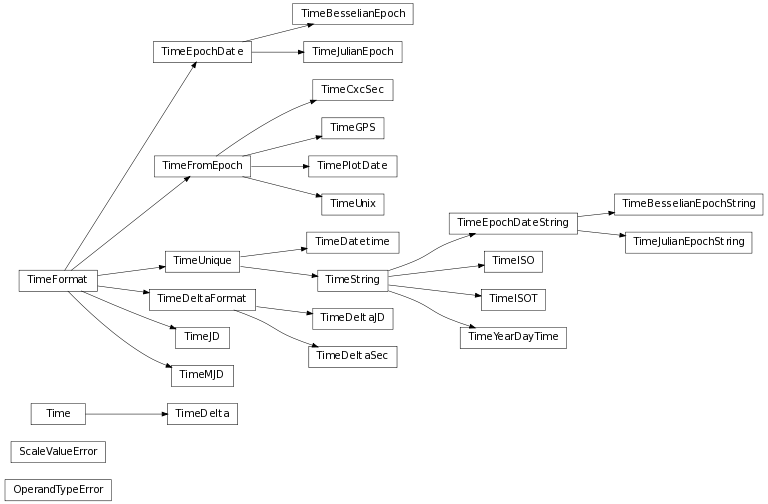
Class Inheritance Diagram¶

Acknowledgments and Licenses¶

This package makes use of the ERFA Software ANSI C library. The copyright of the ERFA software belongs to the NumFOCUS Foundation. The library is made available under the terms of the “BSD-three clauses” license.

The ERFA library is derived, with permission, from the International Astronomical Union’s “Standards of Fundamental Astronomy” library, available from http://www.iausofa.org.

Navigation

Time and Dates (astropy.time)¶